Stochastic Geometry and its Applications, 3^rd edition (2013)

by Chiu, Stoyan, Kendall and Mecke [*]

[*] Our dear colleague and co-author, Joseph Mecke, passed away on 20 February 2014.

 

The purpose of this web page is to inform the reader about points around the book, new ideas and references, as well as errors and typos. We invite you to send your comments, reviews and critiques to us.

 

Send an email message to the authors by clicking here.

 

Order a copy from Wiley, Amazon.

 

Further Remarks, Comments and References:

1.           Page XXI, line -7:

Excellent books on shape include:

a.     Small, C. G. (1996). The Statistical Theory of Shape. Springer-Verlag, New York

b.     Dryden, I. L. and Mardia, K. V. (1998). Statistical Shape Analysis. John Wiley & Sons Ltd, Chichester.

c.      Ghosh, P. K. and Deguchi, K. (2008): Mathematics of Shape Description. A Morphological Approach to Image Processing and Computer Graphics. John Wiley & Sons (Asia) Pte Ltd, Singapore.

d.     Kendall, D. G., Barden, D., Carne, T. K., and Le, H. (1999). Shape and Shape Theory. John Wiley & Sons Ltd, Chichester.

e.      Lele, S. R. and Richtsmeier, J. T. (2001). An Invariant Approach toStatistical Analysis of Shapes. Chapman & Hall/CRC, Boca Raton.

 

2.           Page 27, before Section 1.9:

A function as  can be defined also for non-convex sets, in the spirit of equation (1.52). Examples for thread-like and film-like sets are considered on Ciccariello et al. (2016).

 

Reference:

Ciccariello, S., Riello, P., and Benedetti, A. (2016). Small-angle scattering behavior of thread-like and film-like systems. J. Appl. Crystallography. 49, 260-276.

 

3.           Page 51, Section 2.4:

Another important property of Poisson processes is given by the mapping theorem, which says that under some weak conditions, mappings of state spaces retain the property that a point process is a Poisson process, see Kingman (1993, pp.17-21). An application of the mapping theorem leads to the result that the projection of a Poisson process with an absolutely continuous intensity function from a higher-dimensional space to a lower dimensional one is still a Poisson process, whose intensity function can be obtained by integrating out the unused variables.

 

Reference

Kingman (1993): given on page 477 of the book.

 

4.     Page 67, line -6:

Add Ostoja-Starzewski and Stahl (2000) to the list of references there.

 

Reference

Ostoja-Starzewski, M. and Sthal, D. C. (2000). Random fiber networks and special elastic orthotropy of paper. J. Elasticity 60, 131-149.

 

5.           Page 90, equation (3.106):

The set  is called the difference body of .

 

6.           Page 99, add to the end:

Estimation method for model which can be simulated

Baaske et al. (2014) suggested a general parameter-estimation method based on simulations, which can be applied for the Boolean model, but which is much more general.

The idea is to use some summary characteristic Z that depends on the parameter of interest and then find the parameter that minimises the difference between the values of the empirical and simulated summary characteristics. It is possible to include in the simulation the used sampling method. Geostatistical ideas are used for interpolation.

For the particular case of a planar Boolean model with deterministic discs as grains of radius R the summary characteristic Z was chosen as (A_A, L_A, N_A) and the parameter is (λ, R). The authors found that only the density method based on (3.122) and (3.123) with exactly measured lengths and areas can compete with the simulation-based approach.

 

Reference

Baaske, M., Ballani, F., and van den Boogaart, K.G. (2014). A quasi-likelihood approach to parameter estimation for simulatable statistical models. Image Anal. Stereol. 33, 107-119.

 

7.           Page 120:

Heinrich (2013) defines rigorously what a marked Poisson process is and Baddeley (2010) discusses its properties.

 

References

Baddeley, A. J. (2010). Multivariate and marked point processes. In Gelfand, A. E., Diggle, P. J., Fuentes, M., and Guttorp, P., eds, Handbook of Spatial Statistics, pp. 371-402. CRC Press, Boca Raton.

Heinrich, L. (2013). Asymptotic methods in statistics of random point processes. In Spodarev, E., ed., Stochastic Geometry, Spatial Statistics and Random Fields, Lecture Notes in Mathematics 2068, pp. 115-150. Springer-Verlag, Berlin.

 

8.           Page 134, Section 4.4.7, the second line:

Add the reference Heinrich (2013) after Hanisch (1982).

 

Reference

Heinrich, L. (2013). Asymptotic methods in statistics of random point processes. In Spodarev, E., ed., Stochastic Geometry, Spatial Statistics and Random Fields, Lecture Notes in Mathematics 2068, pp. 115-150. Springer-Verlag, Berlin.

 

9.           Page 145, Section 4.7.1:

Asymptotic s in the theory of point process statistics is thoroughly discussed in Heinrich (2013).

 

Reference

Heinrich, L. (2013). Asymptotic methods in statistics of random point processes. In Spodarev, E., ed., Stochastic Geometry, Spatial Statistics and Random Fields, Lecture Notes in Mathematics 2068, pp. 115-150. Springer-Verlag, Berlin.

 

10.      Page 168, lines -8 and -9:

Add one reference: Voss et al. (2010) à Voss et al. (2010, 2013)

 

Reference

Voss, F., Gloaguen, C., and Schmidt, V. (2013). Random tessellations and Cox processes. In Spodarev, E., ed., Stochastic Geometry, Spatial Statistics and Random Fields, Lecture Notes in Mathematics 2068, pp. 115-150. Springer-Verlag, Berlin.

 

11.      Page 190,

(i)                after formula (5.83), add:

Stucki and Schuhmacher (2014) obtained the following bounds

 

(ii)             after the last line, add:

Following Mase’s suggestion, Stucki and Schuhmacher (2014) derived bounds for H_s(r), D(r) and K(r).

 

Reference

Stucki, K. and Schuhmacher, D. (2014). Bounds for the probability generating functional of a Gibbs point process. Adv. Appl. Prob. 46, 21-34.

 

12.      Page 200, Section 5.6:

Shot-noise random fields play an important role in computer graphics and image processing, where they go under the term spot noise, which was introduced by van Wijk (1991), see also Holten et al. (2006) and Galerne et al. (2011). They serve as models of textures (mostly modeled by stationary random fields). Spot noise is also used for simulating Gaussian random fields, through the use of a localised grain, called a texton, see Galerne et al. (2014).

 

References

Galerne, B., Gousseau, Y. and Morel, J.-M. (2011). Random phase textures: theory and synthesis. IEEE Trans. Image Processing 20, 257-267.

Galerne, B., Leclaire, A. and Moisan, L. (2014). A texton for fast and flexible Gaussian texture synthesis. In 2014 Proceedings of the 22^nd  European Signal Processing Conference, 1-5 September 2014, Lisbon, Portugal, pp. 1686-1690.

Holten, D., van Wijk, J. J. and Martens, J.-B. (2006). A perceptually based spectral model for isotropic textures. ACM Trans. Appl. Perception 3, 376-398.

van Wijk, J.J. (1991). Spot noise: Texture synthesis for data visualization. ACM SIGGRAPH Computer Graphics 25, 309-318.

 

13.      Page 210, lines 14-15:

 

14.      Page 213, after line 6, add the following:

For point processes, Błaszczyszyn and Yogeshwaran (2014) propose a way to use the void probabilities and factorial moment measures to compare variability properties (the degree of clustering) of processes with equal intensity, e.g. Cox processes.

 

Reference

Błaszczyszyn, B. and Yogeshwaran, D. (2014). On comparison of clustering properties of point processes. Adv. Appl. Prob. 46, 1-20.

 

15.      Page 215, the fourth line in the last paragraph of Section 6.2.1, after the word “respectively”, add the following:

In the latter paper the Gibbs distribution is interpreted as a weighted version of the distribution of the typical Poisson polygon or polyhedron, see pages 371 and 374. Figure 6.A shows typical realisations of the Poisson polygon/polyhedron (unweighted) and of a weighted version which prefers circular/spherical shapes. The authors described statistical methods for the estimation of model parameters.

 

(a)	(b)
(c)	(d)

Figure 6.A    Realisations of (a) unweighted Poisson polygons, (b) weighted Poisson polygons, (c) unweighted Poisson polyhedral, and (d) weighted Poisson polyhedral.

 

16.      Page 215, end of Section 6.2.2, add:

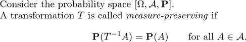
Aggregates of agglomerating particles

Random sets formed by aggregation of (spherical) primary particles play an important role in particle technology, chemistry and physics. A classical model was developed by Smoluchowski (1917), which is based on Brownian motion and contact rules for colliding primary particles.

 

(a)

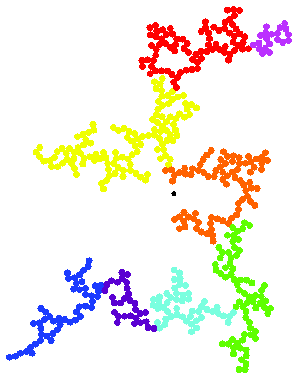
(b)

Figure 6.B    Sample agglomerates from (a) single particle aggregation and (b) cluster-cluster particle aggregation.  Reproduced from Teichmann and van den Boogaart (2015, Figure 3).

 

 

Figure 6.B shows two typical planar aggregates, which are simulated according to a simpler model in Teichmann and van den Boogaart (2015), in which three-dimensional sets are also considered. The distribution of random compact sets of such a nature is probably best described by means of characteristics which see such a particle from its centre of gravity as e.g. the distribution of the distances of the primary particles from this centre. The coordination number distribution of the primary particles also gives valuable insight into the particle structure. The authors also study empirical data, which is available via this link.

 

References

Teichmann, J. and van den Boogaart, K.G. (2015) Cluster models for random particle aggregates—Morphological statistics and collision distance. Spatial Statistics 12, 65-80.

von Smoluchowski, M. (1917) Versuch einer mathematischen Theorie der Koagulationskinetik kolloider Lösungen. Z. Phys. Chem. 92, 129-168. 

 

17.      Page 229, end of Section 6.3.6:

It is useful to consider random-set characteristics that are combined of densities. Of particular interest are the structure model index

f_SMI = 12 V_V M_V / S_V²

and the trabecular bone pattern factor

f_TBPF = M_V / S_V,

which were both developed in the context of analysis of bone structures, but are of much wider interest. See Hahn et al. (1992), Hildenbrand and Rüegsegger (1997) and Ohser et al. (2009).

The former one is a dimensionless “shape factor”, which takes for germ‑grain models of non-overlapping constant spheres, cylinders or plates the values 4, 3 and 0, respectively. The latter is scale-dependent and equals, for germ‑grain models with non-overlapping convex grains, the ratio  / . It can be interpreted as the mean curvature in the typical surface point of X.

Both characteristics have the property to change the sign if applied to the complement of X. For systems of holes they take negative values.

 

References

Hahn, M., Vogel, M., Pompesius-Kempa, M., and Delling, G. (1992). Trabecular bone pattern factor—a new parameter for simple quantification of bone microarchitecture. Bone 13, 327-330.

Hildenbrand, T. and Rüegsegger, P. (1997). A new method for the model-independent assessment of thickness in three-dimensional images. J. Microsc. 185, 67-75.

Ohser, J., Redenbach, C., and Schladitz, K. (2009). Mesh free estimation of the structure model index. Image Anal. Stereol. 28, 179-183.

 

18.      Page 241, equation (6.103):

A distribution with a density function as in (6.103) is called half normal distribution.

 

19.      Page 243, before the subsection on The Stienen model:

Klatt and Torquato (2014) used Voronoi tessellations for the statistical characterisation of hard ball packings. They stated that the distributions of the Minkowski functionals of single cells are not suitable for the characterisation of jammed packings of identical balls. In order to characterise the spatial structure of such Voronoi tessellations they also employed mark correlation functions, where the points are the ball centres and the marks the Minkowski functionals of the corresponding cells, as in Stoyan and Hermann (1986).

 

References

Klatt, M. A. and Torquato, S. (2014). Characterization of maximally random jammed sphere packings: Voronoi correlation functions. Phys. Rev. E 90, 052120.

Stoyan, D. and Hermann, H. (1986). Some methods for statistical analysis of planar random tessellations. Statistics 17, 407-420.

 

20.      Page 244, 4 lines from bottom:

The property that each ball is in touch with a ball of equal or smaller size is known as the smaller-grain-neighbour property.

 

21.      Page 245, before Section 6.5.4

       Engineers study random systems of moving particles. These particles can be hard or soft. They can have contacts or collisions, where physical forces act. A modern source to the literature is the book Nikrityuk and Meyer (2014). There for example the following problems are studied: the breaking dam problem and the behaviour of rolling particles in a rotating drum. All is based on physically founded simulation programs.

       An important, frequently studied problem is the radial porosity in packed beds of balls. Imagine a long cylinder filled with hard balls of constant radius. Consider then a random point within the cylinder of distance r from the boundary of the cylinder. The probability that this point is not within one of the balls is the value of radial porosity e(r). Mueller (2010) contains very precise (empirically found) formulae for e(r)

 

References:

Mueller, G. E. (2010). Radial porosity in packed beds of spheres. Powder Technology 203, 626-633.

Nikrityuk, P. A. and Meyer, B. eds (2014). Gasification Processes: Modeling and Simulation. Wiley-VCH, Weinheim.

 

22.      Pages 266-269, Example 6.6:

The heather example is perhaps not fully perfect.

a.     The estimates for A_A and N_A are not in full agreement with the theory: if A_A = 0.5, then the equality N_A = 0 follows. However, the values given on page 267, last line, are only statistical estimates.

b.     Dr. Felix Ballani carried out goodness-of-fit tests as mentioned on page 269, using the spherical contact distribution function and Mecke’s morphological functions related to L_A and N_A. He found that the model is accepted by the first two functions but not by the third. For small r (r < 0.2 m) the empirical function lies outside simulated envelopes.

Note in passing that Figure 6.14 shows a smoothed version of the heather data, while the estimates come from the original data.

 

23.      Page 269, add the following to the end:

Intensity functions for non-stationary random measures

In analogy to the intensity function L(x) of a point process, one can define an intensity function for a non-stationary random measure that is absolutely continuous with respect to a Hausdorff measure of suitable dimensions. This includes the cases of fibre and surface processes. The paper Camerlenghi et al. (2014) discusses such functions under the name mean density and studies correspponding kernel estimators.

 

Reference

Camerlenghi, F., Capasso, V., and Villa, E. (2014). On the estimation of the mean density of random closed sets. J. Multivariate Anal. 125, 65-88.

 

24.      Page 332:

Redenbach and Thäle (2013) studied g(r) for the segment process of edges of the Poisson-Voronoi tessellation and other tessellations.

 

Reference

Redenbach, C. and Thäle, C. (2013). Second-order comparison of three fundamental tessellation models. Statistics 47, 237-257.

 

25.      Page 333, line 12:

A further reference is Ciccariello et al. (2016).

 

Reference:

Ciccariello, S., Riello, P., and Benedetti, A. (2016). Small-angle scattering behavior of thread-like and film-like systems. J. Appl. Crystallography. 49, 260-276.

 

26.      Page 333, add to the end of the second paragraph:

The paper Redenbach et al. (2014) contains formulae for pair correlation functions for some spatial fibre processes: Poisson line process and edge systems of Poisson hyperplane and STIT tessellations. For the edge system of the Poisson Voronoi tessellation an approximation is presented, which was obtained by the Cox-process method mentioned on page 330. This function is similar to the functions shown in Figure 9.12.

Systems of thick fibres that do not overlap are considered in Altendorf and Jeulin (2011) and Gaiselmann et al. (2013). For their simulation collective rearrangement algorithms are used.

 

References

Altendorf, H. and Jeulin, D. (2011). Random-wallk based stochastic modeling of three-dimensional fiber systems. Phys. Rev. E 83, 041804.

Gaiselmann, G., Froning, D., Tötzke, C., Quick, C., Manke, I., Lehnert, W., and Schmidt, V. (2013) Stochastic 3D modeling of non-woven materials with wet-proofing agent. Int. J. Hydrogen Energy 38, 8448-8460.

Redenbach, C., Ohser, J., and Moghiseh, A. (2014). Second-order characteristics of the edge system of random tessellations and the PPI value of foams. Methodol. Comput. Appl. Probab., DOI: 10.1007/s11009-014-9403-x

 

27.      Page 338, end of Example 8.5:

Ciccariello et al. (2016) contains formulae in its section 3.4.3 that enable the determination of second-order characteristics for the case of a Boolean model with rectangular surface pieces.

 

Reference:

Ciccariello, S., Riello, P., and Benedetti, A. (2016). Small-angle scattering behavior of thread-like and film-like systems. J. Appl. Crystallography. 49, 260-276.

 

28.      Page 338, add to the end of line -10:

Such surfaces are systematically studied in Stoyan (2014). They are of practical interest in the context of interfaces between fluids and porous substrates modeled by hard-ball systems.

 

Reference

Stoyan, D. (2014). Surfaces of hard-sphere systems. Image Anal. Stereol. 33, 225-229.

 

29.      Page 351 line 5 and page 390 Section 9.10.1:

Alpers et al. (2015) and Teferra and Graham-Brady (2015) considered independently an important representation problem for planar and spatial tessellations, which is very important in the context of polycrystalline structures. A tessellation is described by a marked point process with nucleation sites (nuclei) as points and parameters describing growth (speed and geometry of growth) as marks. For example, growth may be ellipsoidal. The determination of the parameters is based on some optimisation procedure. The corresponding tessellations can be constructed by standard techniques. Usually their cell boundaries are curved on the plane and non-planar in space.

Note the use of the term “representation”. This approach does not claim to describe the physical processes leading to polycrystalline structures. For this purpose perhaps (much more complicated) models in the spirit of Johnson-Mehl models may be suitable.

Two teams, one formed by Andreas Alpers, Fabian Klemm and Peter Gritzmann, and the other by Kirubel Teferra, helped the authors of this book to carry out the following experiment: Using as data Figure 9.7 on page 353, which shows a Johnson-Mehl tessellation, the two teams reconstructed the tessellations with their programs independently. The better result was obtained by Alpers, Klemm and Gritzmann shown in Figure 9.A. Each cell here is described by 4 parameters (cell volume, lengths of the semiaxes, and rotation angle of the principal component ellipsoid of the cell) plus the coordinates of the centres of gravity. These parameters were determined as described in Section 3 of Alpers et al. (2015).

 

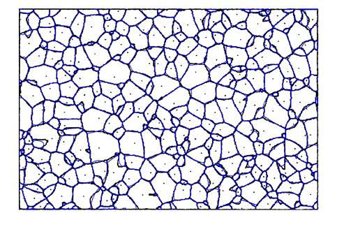
Figure 9.A         A tessellation reconstructed from Figure 9.7 by using the representation in Alpers et al. (2015).  Courtesy of A. Alpers, F. Klemm and P. Gritzmann.

 

The power of the algorithm of Alpers et al. (2015) is impressive: Though the tessellation in Figure 9.7 results from a process in which growth in the sites starts subsequently, the representation belongs to a model in which all sites start at the same instant!

 

References:

Alpers, A., Brieden, A., Gritzmann, P., Lyckegaard, A., and Poulsen, H. F. (2015). Generalized balanced power diagrams for 3D representations of polycrystals. Philosophical Magazine 95, 1016-1028.

Teferra, K. and Graham-Brady, L. (2015). Tessellation growth models for polycrystalline microstructures. Computational Materials Science 102, 57-67.

 

30.      Page 352:

Another name for the Voronoi S-tessellation is Set Voronoi diagram, as used in Schaller et al. (2013). In that paper the tessellation is defined with respect to the three-dimensional assemblies of arbitrary particles. This idea is already appeared in mathematical morphology, see Lantuejoul (1978b) and Preteux (1992). Figure 9.B shows the S-tessellations relative to a system of ellipses and a system of ellipsoids.

 

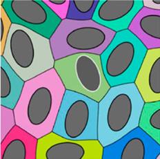
(a)

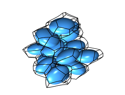
(b)

Figure 9.B                   (a) A planar S-tessellation relative to a system of ellipses and (b) a spatial S-tessellation relative to a system of ellipsoids. Courtesy of G. Schröder-Turk.

 

References

Lantuejoul (1978b): given on page 479.

Preteux, E. (1992). Watershed and skeleton by influence zones: a distance-based approach. J. Math. Imaging Vis. 1, 239-255.

Schaller, F. M., Kapfer, S. C., Evans, M. E., Hoffmann, M. J. F., Aste, T., Saadatfar, M., Mecke, K., Delaney, G. W., and Schröder-Turk, G. E. (2013). Set Voronoi diagrams of 3D assemblies of aspherical particles. Phil. Mag. 93, 3993-4017.

 

31.      Page 352, line -1:

Cowan and Thäle (2014) introduced three more parameters, namely, the probabilities that the typical edge is a side of zero, one and two cells and established further mean-value formulae for tessellations that are not side-to-side.

 

Reference

Cowan, R. and Thäle, C. (2014). The character of planar tessellations which are not side-to-side.  Image Anal. Stereol. 33, 39-54.

 

32.      Page 354, before the subsection on Crack and STIT tessellation:

The tessellations (Voronoi, Laguerre, Johnson-Mehl) discussed so far are based on circular/spherical growth or topology around the generating points. Jeulin (2014) generalised this to other topologies, e.g. with ellipsoidal unit spheres. Even more general are constructions based on random fields, generating points and watershed construction. The paper Altendorf et al. (2014) presents applications to polycrystalline materials.

 

References

Jeulin, D. (2014). Random tessellations generated by Boolean random functions. Pattern Recogn. Lett. 47, 139-146.

Altendorf, H., Latourte, F., Jeulin, D., Faessel, M., and Saintoyant, L. (2014). 3D reconstruction of a multiscale microstructure by anisotropic tessellation models. Image Anal. Stereol. 33, 121-130.

 

33.      Page 386, before Section 9.8:

The limiting distributions of various extreme values, such as the minimum and the maximum of the circumradii or the minimum and the maximum of the areas of Poisson-Delaunay triangles observed in a bounded window are studied in Chenavier (2014). It shows that the triangle having the largest area tends to be equilateral.

 

Reference

Chenavier, N. (2014). A general study of extremes of stationary tessellations with examples. Stoch. Process. Appl., DOI: 10.1016/j.spa.2014.04.009.

 

34.      Page 396, Example 9.4:

The Laguerre tessellation does not yield the observed edge length distributions of foams. Kraynik (2006) reports that better results are obtained if the Laguerre tessellation is annealed by the surface evolver.

 

Reference

Kraynik, A. M. (2006). The structure of random foam. Adv. Eng. Mater. 8, 900-906.

 

35.      Page 398, lines 9-10:

after Sok et al. (2002) and before van Dalen et al. (2007), add: Vogel (2002)

 

Reference

Vogel (2002): given on page 502 of the book.

 

36.      Page 400, after formula (9.145), add:

The variance  of the degree distribution {} is also a useful topological characteristic.

 

37.      Pages 425-436, Section 10.4 (a note of sampling methods as in Section 10.4.3 and Section 10.4.4):

Thórisdóttir and Kiderlen (2013) considered a local approach to the Wicksell problem. Each ball is assumed to contain a reference point (which is not the centre, otherwise the problem would be trivial) and the individual ball is sampled with an isotropic random plane through its reference point. Both the section circle and the position of the reference point in the profile are recorded and used to estimate the ball radius distribution.

 

Reference

Thórisdóttir, Ó. and Kiderlen, M. (2013). Wicksell's problem in local stereology. Adv. Appl. Prob. 45, 925-944.

 

38.      Page 444, the end of Section 10.6:

Redenbach et al. (2014) showed by simulation that S_V can be approximated bycρ₁, where ρ₁ is the radius of the first interference ring of the power spectrum of the length measure of the edge system in a random tessellation. However, the parameter c is not a universal constant for all models.  Nevertheless, it is empirically stable in realisations from the same model or samples of the same material.

 

Reference

Redenbach, C., Ohser, J., and Moghiseh, A. (2014). Second-order characteristics of the edge system of random tessellations and the PPI value of foams. Methodol. Comput. Appl. Probab., DOI: 10.1007/s11009-014-9403-x

 

 

 

 

Typos and Corrections:

1.           Page 167, equations (5.28) and (5.29): The capital L is used to denote a random intensity function in these two equations, but L is also used to denote a deterministic intensity measure or a realisation of the random measure Y on page 166, around equation (5.25). Thus, to avoid confusion, the following changes should be made:

(a)  Four lines above equation (5.28):

“However, such a field cannot be used as the intensity field of a Cox process since it can take negative values.” à “However, the integral of such a field  cannot be used as the driving random measure Y(B) of a Cox process since Z(x) can take negative values.”

(b) One line above equation (5.28), after “in a mathematically tractable model, is”, add the following words:

taking exp(Z(x)) as the random intensity function, i.e.

(c)  Equation (5.28) should be:

(d) Two lines above equation (5.29):

“The random intensity of…” à “The random driving measure of…”

(e)  Equation (5.29) should be:

 

2.           Page 233, equation (6.87): the denominator should be

 

3.           Page 262, equation (6.157): it should be

 

4.           Page 374, Table 9.3, the last row, the second to last column: in the expression for the cross-product moment between N and , the denominator should be 24r, instead of 12r, i.e.

 

Table 9.3  …

…

 

The original incorrect expression was taken from Santaló (1976, p.297) [who referred to Miles (1973); however, it seems these formulae came from Miles (1972b, p.252)]. The mistake probably was caused by the difference in the parameters: In our notation, Santaló used r (the mean number of planes intersected by a test line segment of unit length) while Miles used S_V (the intensity of the Poisson plane process).  The denominator of the corresponding expression in Miles (1972b) is 12S_V, which is equal to 24r, but Santaló forgot to change 12 to 24 after reparametrisation; nevertheless, the other expressions for the moments in Santaló (1976) agree with Miles (1972b).

 

5.           Page 430, equation (10.50): The n in the denominator on the right-hand side should be replaced by p.

 

6.           Page 457, line 25: The bibliographical detail of the reference Ballani and van den Boogaart (2013) is

Ballani and van den Boogaart (2014), Methodol. Comput. Appl. Probab. 16, 369-384.

 

7.           Page 461, line -3: The bibliographical detail of Chiu and Liu (2013) is

Biometrics 69, 497-507.

 

8.           Page 468, line 27: The bibliographical detail of Ghorbani (2012) is

Ghorbani, M. (2013).  Metrika 76, 697-706.

 

9.           Page 469, lines -1 and -2: The reference Gille (2014) should be

Gille, W. (2014). Particle and Particle Systems Characterization: Small-Angle Scattering (SAS) Applications. CRC, Boca Raton.

 

10.      Page 486, line 8: The publication year of the reference Molchanov and Stoyan (1995) should be 1996, instead of 1995.